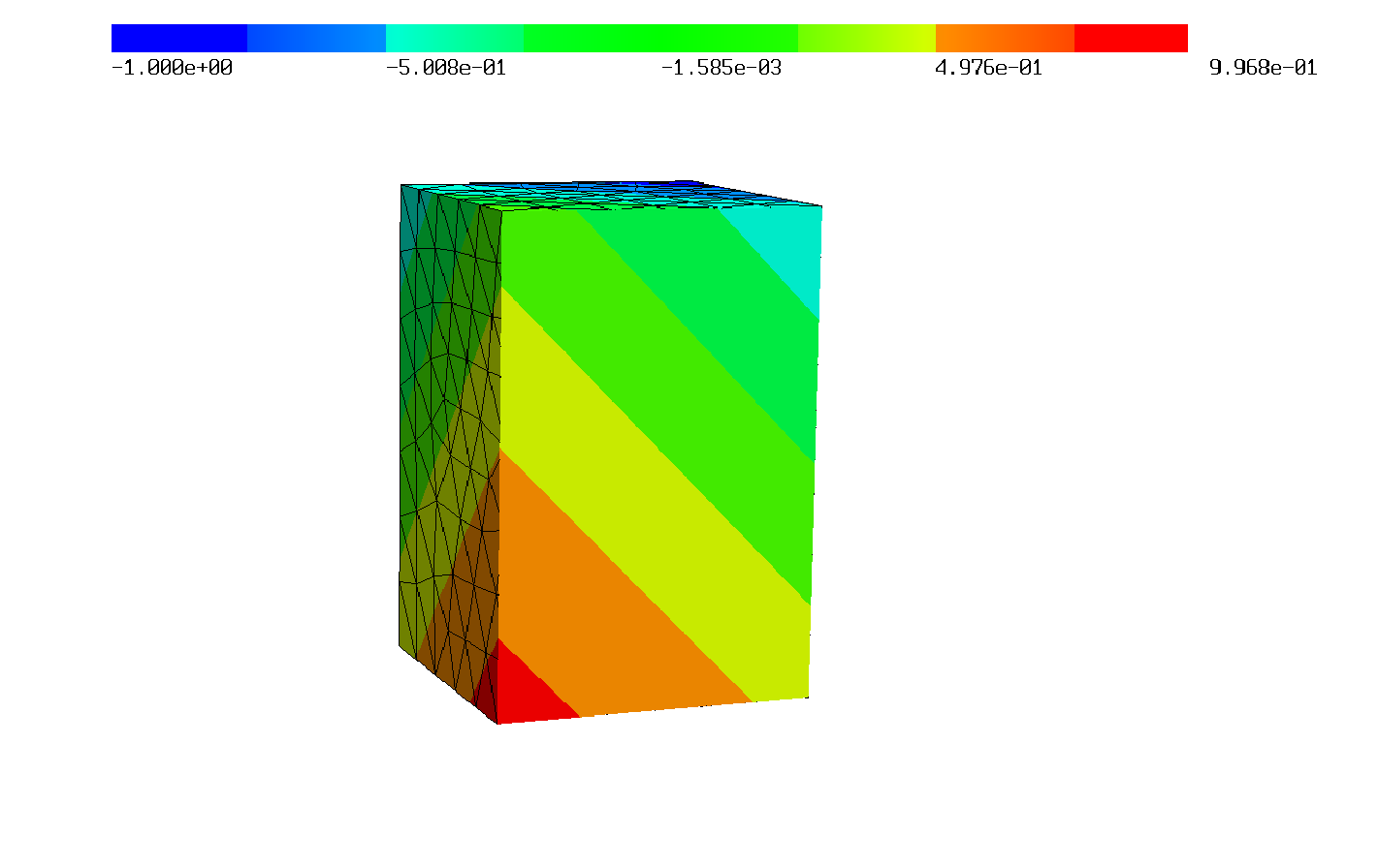
We can now define generic (quasi-)periodic finite element spaces which work for all the main function spaces (H1, HCurl, HDiv, and maybe some others...) by creating a finite element space wrapper with a mapping of the degrees of freedom. This wrapper is created from python by calling the generator function Periodic.
The generator function can create periodic as well as quasiperiodic spaces where the slave boundary is equal to the master boundary up to a phase shift (usually a complex constant with norm 1). Here I want to show how to use this, to solve the problem:
Find \( u \in H^1_{qp} \) such that \[ \int_\Omega \nabla u \nabla v + uv \, dx = \int_\Omega (k^2+1) e^{ik d\cdot x} v \, dx \] for all \( v \in H^1_{qp} \) ,where \[ \Omega = (0,Lx) \times (0,Ly) \times (0,Lz), \] \( k \) is the wave number, \( d \) the incoming wave direction and \( H^1_{qp} \) the quasi periodic \( H^1 \) space with phase shifts \[ (fx,fy,fz) = (e^{ik d_x Lx}, e^{ik d_y Ly}, e^{ik d_z Ly}). \] Obviously \[ u = e^{ik d \cdot x} \] solves this problem.
We choose the variables as
k=1.
Lx=1.
Ly=2.
Lz=1.5
d=[1./sqrt(3),1./sqrt(3),1./sqrt(3)]
Creating the geometry and specifying the periodic surfaces for the mesh:
geo = CSGeometry()

left = Plane(Pnt(0,0,0),Vec(-1,0,0))
right = Plane(Pnt(Lx,0,0),Vec(1,0,0))
bot = Plane(Pnt(0,0,0),Vec(0,0,-1))
top = Plane(Pnt(0,0,Lz),Vec(0,0,1))
back = Plane(Pnt(0,0,0),Vec(0,-1,0))
front = Plane(Pnt(0,Ly,0),Vec(0,1,0))

cube = left * right * top * bot * back * front

geo.Add(cube)
geo.PeriodicSurfaces(left,right)
geo.PeriodicSurfaces(back,front)
geo.PeriodicSurfaces(bot,top)
Define the factors and create the quasiperiodic FESpace:
fx = exp(1J*k*d[0]*Lx)
fy = exp(1J*k*d[1]*Ly)
fz = exp(1J*k*d[2]*Lz)
factors = [fx,fy,fz]
fes = Periodic(H1(mesh,order=5,complex=True),phase=factors)
The problem is then set up and solved in the usual way:
a = BilinearForm(fes)
a += SymbolicBFI(grad(fes.TrialFunction()) * grad(fes.TestFunction()) + fes.TrialFunction() * fes.TestFunction())
f = LinearForm(fes)
f += SymbolicLFI((k**2+1)*exp(1J*k*(d[0]*x+d[1]*y+d[2]*z)) * fes.TestFunction())

u = GridFunction(fes,name="u")

with TaskManager():
    a.Assemble()
    f.Assemble()
    u.vec.data = a.mat.Inverse(fes.FreeDofs()) * f.vec

Draw(u)
Finally we compare our solution to the true solution:
u_true = exp(1J * k * (d[0] * x + d[1] * y + d[2] * z))
print("error: ", sqrt(Integrate(Conj(u_true-u)*(u_true-u),mesh).real))
This gives:
error: 8.096041963840607e-11
 If you go into the "Visual" menu and activate "Animate periodic" you can see the wave travel.

